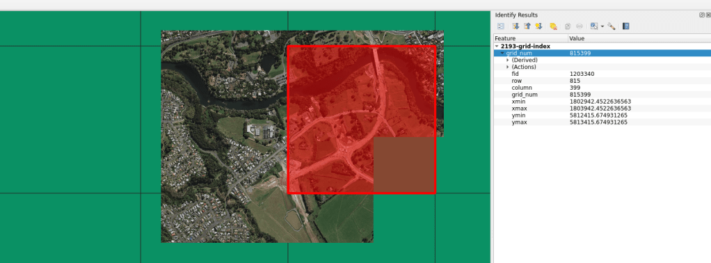
Static Vector Tiles for Small Projects

Contours Wellington

Update 04/05/2021: This method has been improved and found here.

The following covers a method for visualizing a complex vector tile dataset using a static server.  This particular blog is more for beginners and reduces the technical terms as much as possible. I wouldn’t recommend this method for large complex vector tile data sets, but instead for quick one-off sites that are looking to incorporate a small number of vector tiles where the GeoJSON might be too large/complex to handle.

If you just want to skip to the map and code, visit the Github page created for this blog.

Here is the big reveal at the beginning. If you want to serve a basic vector tile locally or with a static server:

  1. Create an tile cache with uncompressed .pbf files
  2. Place that tile cache on something like GitPages, e.g. embed the tile cache directly along with your website or embed the cache on your localhost along with the other site files
  3. In Leaflet, access the tile cache using ‘L.vectorGrid.protobuf()’

If you’d like to read more in depth:

I work on a Ubuntu OS; however, the methods below will just as easily work with iOS and Windows environments. The parts for building the site, e.g. the HTML, JS, CSS and GitPages, are OS agnostic.

If you want to follow the steps outlined you will need to have installed:

  • GDAL: I am only including this since I used GDAL to extract the contours from the original elevation file.
  • OGR2OGR: Easy tool for converting your shapefile to GeoJSON.
  • Tippecanoe: Excellent tool for generating your tile caches in Web Mercator.
  • T-Rex: Necessary for building your tile cache in a custom projection like NZTM. I tried a number of methods and T-Rex seemed to work best. Sadly, as of Nov 2020, ogr2ogr cannot currently create an MVT in NZTM projection, but it can do projections where the resolutions are halved at each zoom level.
  • Leaflet: Your friendly JS library for building your map in a web environment.
  • SimpleHTTPServer: if you’d like to do localhost testing, you can run your site with this.

You will also need a Github account and a basic knowledge of building a webpage .

Here are the two stacks depending on your needs:

  • Web Mercator: GDAL, OGR2OGR, Tippecanoe, Leaflet, GitPages
  • NZTM: GDAL, OGR2OGR, PostGIS, T-Rex, Leaflet, GitPages

The basic premise is this: with your vector file, you need to construct a tile cache with uncompressed PBF files. The tile cache is the same as any XYZ tile cache you would use for raster tiles, except you are filling it with .pbf files. That tile cache will need to reside in a location accessible by your Leaflet application. In this example we are using GitPages as our server and embedding our tiles directly along with the website we built. Technically, Gitpages is acting as the server. If you are testing and serving on localhost, just embed your tile cache with your web files.

I am going to keep the code light for this blog and instead layout the steps. You can find full code examples in my Github repository here.

Building Your Own Contours

Download Elevation in NZTM
https://data.linz.govt.nz/layer/53621-wellington-lidar-1m-dem-2013/

If you download the entire dataset, you can create the contour lines from the VRT. This saves a lot of time by not creating a mosaic.

Build VRT

gdalbuildvrt dem.vrt *.tif

Contour (@ 50m intervals)

gdal_contour -a elev -i 50 dem.vrt wellyDEMContour.shp

Web Mercator Tile Cache

If you are building a Web Mercator site, you can use Tippecanoe to render the tile cache. You need to create a GeoJSON of your shapefile first

Shape to GeoJSON

ogr2ogr -f GeoJSON -a_srs EPSG:2193 -t_srs EPSG:3857 wellyDEMContour.json wellyDEMContour.shp

Tile JSON

tippecanoe --no-tile-compression --projection=EPSG:3857 --minimum-zoom=12 --maximum-zoom=16 --output-to-directory "static.vector.tiles/contoursWebmer" wellyDEMContour.json

NZTM Tile Cache

If you are building an NZTM site you will need to use T-Rex to generate the NZTM tile cache for the vector tiles. T-Rex likes best if you can give it a PostGIS table to work from. I’d also recommend simplifying complex contour data sets. Your tile generation will be much faster.

Upload to PostgreSQL (you can upload the original NZTM shapefile)

shp2pgsql -s 2193 wellyDEMContour_NZTM.shp public.contournztm | psql -h localhost -d dbName -U userName

T-Rex Config

See full config here

Note the tile size you are setting. You will need this later for your Leaflet application

[grid.user]
width = 4096
height = 4096
extent = { minx = -1000000, miny = 3087000, maxx = 3327000, maxy = 10000000 }
srid = 2193
units = "m"
resolutions = [8960.0,4480.0,2240.0,1120.0,560.0,280.0,140.0,70.0,28.0,14.0,7.0,2.8,1.4,0.7,0.28,0.14,0.07]
origin = "TopLeft"

T-Rex Tile Cache

t_rex generate --progress true --maxzoom=12 --minzoom=9 --extent=160.6,-55.95,-171.2,-25.88 --config /static.vector.tiles/trexConfig/configpsql_contour.toml

Decompress PBF Files

find . -type f | xargs -n1 -P 1 -t -I % gzip -d -r -S .pbf %
find . -type f | xargs -n1 -P 1 -t -I % % %.pbf

Important bit for Leaflet

See the GitPages site for how to set up the Leaflet JS in NZTM


// Access the tile cache
var vector = L.vectorGrid.protobuf(vectorURL, styles);

Have fun!

Basic GRASS GIS with BASH, plus GDAL

As a follow-up to the last blog, I thought it would be helpful to demonstrate how next to break up the elevation example into individual watersheds. The reason being, in my last example I demonstrated the process using a square raster tile. Hydrological processes are not accurate when run on square tiles. It is best to run further processes, like stream order extraction, on complete watersheds.

If you are reading this and want to follow along, it is very helpful to go back and read this blog. The following builds off that last example.

I’ll break this into two parts:

1. Creating multiple watershed boundaries of different sizes with GRASS and using a basic loop in BASH for the process.
2. Clipping the original raster by the watershed boundaries using GDAL and SQL with a basic loop in BASH.

Creating Watershed Boundaries with Varying Sizes

This section will modify the script created in the last post.

Notice in the previous script, when I used r.watershed, I set the threshold value to 100000. You can use this value to set the minimum size of your watershed based on cell units. I see this as minimum number of pixels per watershed since your cell unit is the size of your pixel.

threshold=100000
accumulation=${rasterName}_accumulation
drainage=${rasterName}_drainage
stream=${rasterName}_stream
basin=${rasterName}_basin
r.watershed elevation=$fillDEM threshold=$threshold accumulation=$accumulation drainage=$drainage stream=$stream basin=$basin --overwrite

Have a play setting the threshold value to different values, like 2000000 or 5000. You will get very different outputs in your watersheds vector layer. Try to determine the upper most threshold value you can input before GRASS can no longer determine a watershed.

Warning: really small threshold values will take very long to process and give very poor results, like thousands of very tiny watersheds of little to no value in analysis.

Once you have found you upper most limit for you threshold, determine a few lesser values and build them into a list. Maybe take the upper limit, half it, then half it again.

Make that into a list into a variable:

$ list=$(echo 2000000 1000000 500000)

Then loop the list to iterate through your threshold values when running r.watershed in GRASS. All we change from the last script is the threshold value to use the item from the list. Note we add the threshold value as part of the name too.

Use the standard form of a BASH loop:

for i in $list
do
    echo $i 
done

Loop with GRASS watershed commands:

list=$(echo 2000000 1000000 500000)

for i in $list
do
    # Run watershed operation on fill sink raster
    threshold=$i
    accumulation=${rasterName}_accumulation_${i}
    drainage=${rasterName}_drainage_${i}
    stream=${rasterName}_stream_${i}
    basin=${rasterName}_basin_${i}
    r.watershed elevation=$fillDEM threshold=$threshold accumulation=$accumulation drainage=$drainage stream=$stream basin=$basin --overwrite

    # Convert Basin (watershed) to vector format
    basinVect=${rasterName}_basinVect_${i}
    r.to.vect input=$basin output=$basinVect type=area column=bnum --overwrite

    # Export catchment to vector format
    basinVectOut=${outDir}/${rasterName}_basinVectOut_${i}.shp
    v.out.ogr input=$basinVect output=$basinVectOut type=area format=ESRI_Shapefile --overwrite
done

Full script example here

Your outputs this time will be a collection of shapefile watersheds constructed by your threshold value.

Clipping your Raster by Individual Watersheds using GDAL, OGR and SQL

The watersheds layers are full of nice watersheds, however you cannot simply clip the elevation raster by the full vector file. For the clip, you need to select each individual watershed first. The following will demonstrate how to list each of those watersheds and use them as a clip file via a loop.

To start, set up a test directory for your processed raster outputs:

$ mkdir grass_test/raster_watersheds

The basic command for clipping a raster with a vector in GDAL is:

$ gdalwarp -of GTiff -cutline input_shapefile_for cut.shp input_raster_to_be_cut.tif output_raster.tif

You could create a shapefile for each watershed and clip your raster by that watershed individually using the command above, but the process would be fraught with errors and take a very long time.

It is much easier to automate the process using a combination of ogrinfo, sql and gdal.

We’ll do this with an example using JM_basinVectOut_2000000.shp you just created.

JM_basinVectOut_2000000.shp

In the example, we’ll:

1. Read and list individual watersheds from the vector layer, by listing all the ‘cat’ values leveraging the ogrinfo -sql switch.
2. Using the list, we’ll clip the original raster by each individual watershed

First, list the ‘cat’ values in the vector watershed layer.

The basic ogrinfo command is:

$ ogrinfo /grass_test/JM_basinVectOut_2000000.shp

For this operation; however, we need to list the information of each row in the attributes:

$ ogrinfo -geom=NO -q -sql "SELECT cat FROM JM_basinVectOut_2000000" /grass_test/JM_basinVectOut_2000000.shp

In the above ogrinfo command lists all of the rows for the ‘cat’ column, excluding any geographic information for the file. To do this we use the ‘-sql’ switch available in ogrinfo.

Note when using the ‘-sql’ switch you need a layer name, ‘JM_basinVectOut_2000000’ from the shapefile. The layer name is just the name of the shapefile with the .shp removed.

Use grep to select the parts from the output you want and sed to clean up the outputs for a tidy list.

$ ogrinfo -geom=NO -q -sql "SELECT cat FROM JM_basinVectOut_2000000" /home/ireese/grass_test/JM_basinVectOut_2000000.shp | grep 'cat (Integer)' | sed s/'cat (Integer) =//g'

Make it a list variable:

$ watershedList=$(ogrinfo -geom=NO -q -sql "SELECT cat FROM JM_basinVectOut_2000000" /home/ireese/grass_test/JM_basinVectOut_2000000.shp | grep 'cat (Integer)' | sed s/'cat (Integer) =//')

Before we loop the process in gdal lets look quickly at why this list was created.

In gdalwarp we are going to again leverage the ‘-sql’ switch in order to select each individual watershed row and clip only by that row. We’ll be writing the a basic ‘sql’ similar to the above, but instead filtering by each watershed:

SELECT cat FROM watershed WHERE cat=$i

So, putting all the bits together, using clip and SQL, in gdalwarp we get:

$ gdalwarp -of GTiff -dstnodata -9999 -cutline $inputVector -csql "SELECT cat FROM $inputVectorLayerName where cat='$i'" -crop_to_cutline input_raster_to_be_cut.tif output_raster.tif

Note, I am using ‘-crop_to_cutline’ and ‘-dstnodata’. Basically I’m saying, crop the output raster the bounding box of the input vector and set a ‘nodata’ value of -9999 to the pixels outside the clip area.

Now we need put this all together in a script to loop the process.


#!/bin/bash

# set base path
outDir=grass_test
outDirRast=grass_test/raster_watersheds

# Set raster as variable
raster=${outDir}/lds-tile-jm-GTiff/JM.tif
rasterName=$( basename $raster | sed 's/.tif//g' )

#prep your input vectors
inputVector=/home/ireese/grass_test/JM_basinVectOut_2000000.shp
inputVectorLayerName=$(basename $inputVector | sed 's/.shp//')

#create your watersheds list
watershedList=$(ogrinfo -geom=NO -q -sql "SELECT cat FROM $inputVectorLayerName" $inputVector | grep 'cat (Integer)' | sed s/'cat (Integer) = //')

for i in $watershedList
do
    gdalwarp -of GTiff -dstnodata -9999 -cutline $inputVector -csql "SELECT cat FROM $inputVectorLayerName where cat='$i'" -crop_to_cutline $raster $outDirRast/${rasterName}_${i}.tif
done

Copy the above script, check your file paths, and save it in a text editor as:

rasterClipByWatershed.sh


To run the script:

$ bash grass_test/rasterClipByWatershed.sh

Final Note
In the above process, it may be necessary to run some clean up operations to remove invalid geometries in the watersheds vector layer. I did not include this, but it is helpful to resave the watersheds shapefile first by running a buffer operation with a buffer value of ‘0’. This will remove the invalid geometries. You can run this in GRASS or using ogr2ogr with PostGIS. Here is an ogr2ogr with PostGIS example:

$ ogr2ogr -f "ESRI Shapefile" output_vector.shp input_vector.shp -dialect sqlite -sql "select id, ST_buffer(Geometry,0) as geom from input_vector" -overwrite

All the scripts from the past two posts can be found here.

Let me know of this helpful. I could potentially move on to doing some more basic hydro analysis with GRASS and BASH, but these things take time and energy. It would be good to know if these sorts of blogs have value to the wider geospatial world.

Basic GRASS GIS with BASH

I love GRASS… GIS

But this wasn’t always the case.

GRASS GIS was, for a long time, something I dismissed as ‘too complex’ for my everyday geospatial operations. I formulated any number of excuses to work around the software and could not be convinced it had practical use in my daily work. It was ‘too hard to set-up’, ‘never worked well with QGIS’, and ‘made my scripting processes a nightmare’.

I am here to officially say I’ve been very wrong for a very long time. GRASS GIS is pretty amazing and is a wonderfully easy tool to script.

Recently I scripted a model for extracting river centrelines from high resolution elevation data. During the process I thought how useful it would have been, way back, to have a simple example for setting up an environment and scripting a BASH process using GRASS. So, I built one for myself.

The following example provides the steps for a simple catchment extraction on a piece of LINZ 8m elevation data. The example is only for demonstration of running a basic BASH/GRASS set up with a hydrology command and NOT a demonstration for how to do hydrology using GRASS. The 8m elevation data is not the best data for hydrological extraction; however, these data do provide a nicely sized dataset to use as practice and will give results. Also please note, catchment extraction on a square raster is will not give accurate results at the edges of the raster.

In this example we will:

1. Download a small piece of elevation data from the LINZ Data Service
2. Build a GRASS environment to process these data
3. Build a BASH script to process the catchments
4. Import the elevation into the GRASS environment
5. Perform some basic GRASS operations (fill and watershed)
6. Export raster format for viewing
7. Export the vector catchments to shapefile

The following assumes you are working in a Linux environment and have a basic knowledge of BASH scripting. I tested this process using Ubuntu 18.04 and GRASS 7.4. I have 16GB RAM on my machine.

If you do not all ready have it, you can install GRASS as follows:

$ sudo apt-get install grass-core

If interested, but not necessary, you can install functionality for building GRASS plug-ins:

$ sudo apt-get install grass-dev

Create yourself a directory to work in:

$ mkdir grass_test

Download a piece of elevation data from the LINZ Data Service, place in your directory:

https://data.linz.govt.nz/layer/51768-nz-8m-digital-elevation-model-2012/data/

From the Tiles Table, I downloaded the JM tile in EPSG:2193.

Within your directory you will need to build a ‘PERMANENT’ folder in order for GRASS to do its magic. This folder will be set to operate in the projection of your data. Be sure your data is in the same projection as the environment you built. The data is downloaded in EPSG:2193, New Zealand Transverse Mercator (NZTM), so we set the GRASS environment to work in this projection:

$ grass -c epsg:2193 -e grass_test/GRASS_ENV

‘-c’ will create your directory using epsg:2193 and ‘-e’ will exit once this operation is complete.

Running this command will build a PERMANENT folder in:

grass_test/GRASS_ENV

providing all the bits GRASS needs to operate. Your folder structure will look like:

grass_test/GRASS_ENV/PERMANENT

Have a look inside the folder and see what GRASS built for itself.

The key from now on is to always run your BASH script through this environment. Running your script in this environment will allow you to perform BASH and GRASS commands at the same time.

First, let’s look at the the basic command to run a BASH script using a GRASS environment.

$ grass grass_test/GRASS_ENV/PERMANENT --exec sh grass_test/catchment.sh

The above says, launch GRASS using this environment

grass_test/GRASS_ENV/PERMANENT

and execute, –exec, this script

/grass_test/catchment.sh

Let’s build the BASH script. In this we will:

1. Import the elevation data. GRASS likes to work in its own data formats
2. Set the region for where the operation will be performed. GRASS needs to know where the operation is going to be performed.
3. Perform the operations, r.fill.dir and r.watershed
4. Export a raster to .tif format
5. Export the vector outputs to .shp format


#!/bin/bash

# set base path
outDir=grass_test

# Set raster as variable
raster=${outDir}/JM.tif

# Set a base name for the data. This is used to demonstrate that normal
# BASH commands can be used in this process, along side GRASS
rasterName=$( basename $raster | sed 's/.tif//g' )

# Import raster data
r.in.gdal input=$raster output=$rasterName --overwrite

# Set region. IMPORTANT so GRASS knows where the data is located.
# This region is set for the duration of the following commands
g.region rast=$rasterName

# Fill sinks
fillDEM=${rasterName}_filldem
directionDEM=${rasterName}_directiondem
areasDEM=${rasterName}_areasDEM
r.fill.dir input=$rasterName output=$fillDEM direction=$directionDEM areas=$areasDEM --overwrite

# Export a raster for viewing
areaOut=${outDir}/${rasterName}_areas.tif
r.out.gdal input=$areasDEM output=$areaOut

# Run watershed operation on fill sink raster
threshold=100000
accumulation=${rasterName}_accumulation
drainage=${rasterName}_drainage
stream=${rasterName}_stream
basin=${rasterName}_basin
r.watershed elevation=$fillDEM threshold=$threshold accumulation=$accumulation drainage=$drainage stream=$stream basin=$basin --overwrite

# Convert Basin (watershed) to vector format
basinVect=${rasterName}_basinVect
r.to.vect input=$basin output=$basinVect type=area column=bnum --overwrite

# Export catchment to vector format
basinVectOut=${outDir}/${rasterName}_basinVectOut.shp
v.out.ogr input=$basinVect output=$basinVectOut type=area format=ESRI_Shapefile --overwrite

There you have it. A simple BASH script, set up for running some GRASS commands, running on your LINUX machine.

Putting it all together

Set up you environment, copy the above script, paste it into a text editor, save it as:

grass_test/catchment.sh

Now run

$ grass grass_test/GRASS_ENV/PERMANENT —exec sh grass_test/catchment.sh

Your output catchments shapefile should be similar to the image below

wshed_output


Click here for the next step in this process; how to clip your raster using the watershed layer using GDAL and loops.

Let me know if this was helpful or if you would like to see any changes.

Open Source Stack for Raster Tiling in Custom Projections

This post is a high level look at the recent stack I built for a raster tiling set up. I am working out some kinks in my online and network delivery of cartographic products, so I thought it was time to set up a raster tiling service to access XYZ and WTMS services from my raster tile caches. I’ll be adding maps and zooms levels in the future, so check back now and again. Antarctica is on it’s way soon!

nz_from_basemap_service

Basic Demo Service using NZTM projection is here: https://xycarto.github.io/

See below for WMTS links

Raster tiling is not the only method, but it is still a viable choice for delivering nice looking maps online, serving across networks, and designing with raster data. I am particularly enamored with the quality of the visual outputs. For me, it is akin to the difference between music in vinyl and digital formats. In addition, the process is well documented and fairly straight forward. By virtue of having been around for a while, raster tiling has a wealth of information and standards to work with, delivery from S3 is a robust process, and there is nice integration with QGIS, Leaflet and Openlayers.

I break the stack in to three areas: analysis, rendering, and delivery

Analysis
QGIS: Sketching, QC, and general geospatial work.

GDAL: Processing raster data. Configuring your rasters in an optimal format from the beginning will greatly improve your rendering speeds. I recommend creating a good set of overviews and gathering everything into a virtual raster tile (VRT).

Postgres/PostGIS: Handling your vector data. Pulling all your data from a database significantly improves rendering speeds. Don’t forget to index!

Rendering
Tilemill/Mapnik XML: Yes, I still design using CartoCSS when working with raster data. I love the simplicity of the language. Tilemill is easy enough to containerize these days too. Tilemill exports into the Mapnik XML format, essential for my process further down the line. Here is how to hack Tilemill to work in a custom projection.

Mapnik: Support for using Mapnik XML

Mapnik with Python Bindings: Necessary for using Mapnik XML documents in MapProxy

MapProxy: MapProxy is a map server and tile renderer . It is easy to build on your machine, though I recommend using a container like Docker. Specifically, I use a hack provided by PalmerJ at Github to increase rendering speeds through multi-threading.

Delivery
Amazon S3: Simple Storage Service. Amazon is pretty cheap, free in many cases, and a good place for storing your tile cache. You get an easily accessed URL for your tiles and a home for your WMTS GetCapabilities document.

WMTS: For me, the real power in a base map service is the WMTS, so, below are two links to the WTMS service for you to set up in QGIS if you’d like to have a play. Here is a quick tutorial about how to set up WMTS if you are unfamiliar.

https://s3-ap-southeast-2.amazonaws.com/basemaps.temp/nz_colour_basemap/WMTSCapabilities.nz_colour_basemap.xml
https://s3-ap-southeast-2.amazonaws.com/basemaps.temp/nz_topo_basemap/WMTSCapabilities.nz_topo_basemap.xml

XYZ: Building a web map? If your tile cache is in S3, in a TMS structure, and public you should be able to access it via simple XYZ request like so:

https://{s3-your-region-here}/{your_bucket}/{project_name}/{projection}/{z}/{x}/{y}.png

Leaflet: Leaflet will handle all the XYZ requests to the server and allow for custom projections. Have a look here for the basic HTML, CSS and JS set up.

Experimenting with Hydrological Analysis using TauDEM

Blue Rivers Ordered

Over the past few years, I’ve played around with developing ordered rivers networks for different projects. I am not an expert in hydrology, but I can get close for cartographic purposes. I am an expert; however, in asking for help from those who know best and I rely on a lot of very smart people to guide me on my journey.

Recently, I decided to put together a visualization of ordered rivers for New Zealand. I came across a very nice data set offered through the Ministry for the Environment via the Koordinates website and thought I’d like to put it to use.

The rivers vis project made me wonder if I could build this base dataset myself using some of the recently released elevation data sets via the LINZ Data Service. The short answer to my question is “sorta”. Doing it open source is not an issue, but building an accurate ordered river centerline network is another story. This is a task I cannot take on as a solo project right now, but I could do a little experimentation. Below, I’ll offer some of methods and things I learned along the way.

Tools and Data

The method I tested used TauDEM and a 1m DEM raster accessed from the LINZ Data Service. I down sampled the DEM to 2m and 5m resolutions and used small areas for testing. Finding and open source tool was easy. I sorted through a few available methods and finally landed on “Terrain Analysis Using Digital Elevation Models” (TauDEM). There are additional methods through GRASS and SAGA GIS. I chose TauDEM because I never used it before.

Method Tested

To my knowledge, there is no open source tool where a person can put in a DEM and get a networked rivers centerline vector out the other side. It requires a number of steps to achieve your goal.

The basic run down to process the DEM is to:

  1. Fill sinks
  2. Determine flow directions
  3. Determine watersheds
  4. Determine flow accumulation
  5. Stream classification
  6. Export to vector

TauDEM does require a few extra steps to complete the process, but these steps are explained in the documentation of the tool. It was more about keeping all my variables in the right places and using them at the right time. I recommend using the variable names TauDEM provides.

BASH script here

Click the arrow to the left to view the full BASH script below:

#!bin/bash

#Rough sketch for building river centerlines. Rasters have been clipped prior

BASEPATH=/dir/path/to/base

raster_list=$( find $BASEPATH -name "*.tif" )

taudem_outputs=/dir/path/to/outputs

reso=resolution_number

for i in $raster_list
do

	INPUT_RASTER=$i

	file_name=$( basename $i )

	strip_input_extension=$( echo $file_name | sed 's/.tif//' )

	reso_name=$taudem_outputs/${strip_input_extension}_${reso}res

	gdal_translate -tr $reso $reso -of GTiff $i $reso_name.tif

	fel=${reso_name}_fel.tif
	p=${reso_name}_p.tif
	sd8=${reso_name}_sd8.tif
	ad8=${reso_name}_ad8.tif
	ang=${reso_name}_ang.tif
	slp=${reso_name}_slp.tif
	sca=${reso_name}_sca.tif
	sa=${reso_name}_sa.tif
	ssa=${reso_name}_ssa.tif
	src=${reso_name}_src.tif

	ord=${reso_name}_strahlerorder.tif 
	tree=${reso_name}_tree.dat
	coord=${reso_name}_coord.dat
	net=${reso_name}_network.shp
	w=${reso_name}_watershed.tif 

	processed_input_file=$reso_name.tif

	#TauDEM Commands
	mpiexec -n 8 pitremove -z $processed_input_file -fel $fel

	mpiexec -n 8 d8flowdir -fel $fel -p $p -sd8 $sd8 

	mpiexec -n 8 aread8 -p $p -ad8 $ad8 -nc

	mpiexec -n 8 dinfflowdir -fel $fel -ang $ang -slp $slp

	mpiexec -n 8 areadinf -ang $ang -sca $sca -nc

	mpiexec -n 8 slopearea -slp $slp -sca $sca -sa $sa

	mpiexec -n 8 d8flowpathextremeup -p $p -sa $sa -ssa $ssa -nc

	mpiexec -n 8 threshold -ssa $ssa -src $src

	mpiexec -n 8 streamnet -fel $fel -p $p -ad8 $ad8 -src $src -ord $ord -tree $tree -coord $coord -net $net -w $w

done

The script is a rough sketch, but does get results.

Challenges in the Process

One major challenge for this project was the size of the input DEM and my computers available RAM. I work primarily off a laptop. It’s a good machine but no match for a proper server set up with some spacious RAM. My laptop struggled with the large hi-resolution DEMs, so I needed to down-sample the images and choose a smaller test area to get it to work.

Clip the tiff with gdal_translate -projwin and down sample with -tr

gdal_translate -tr xres yres -projwin ulx uly lrx lry input.tif output.tif


The second challenge came up because I used a bounding box to clip my test regions. I recommend not doing this and instead clip your regions using a watershed boundary. Having square shapes for your test regions will give you very inaccurate and unhelpful results. For example, major channels in your DEM will be cut at the edges of your raster. You will not get accurate results.

Clipping a raster using a shapefile, like a watershed boundary, can be achieved using gdalwarp.

gdalwarp –cutline input.shp input.tif output.tif


Results

I ran my process and QCed the results against Aerial Imagery and a hillshade I developed from the DEM. The first run gave me good enough results to know I have a lot of work to do, but I did manage to develop a process I was happy with. The tool did a great job, but the accuracy of the DEM was a little more challenging. It’s a start. I captured a good number of river channels despite my incorrect usage of a square DEM, learned a lot about how DEM resolution affects outputs, and gained knowledge around how to spot troublesome artifacts.

Well Defined ChannelsImg 1: River capture in well defined channel.

From this experiment, there are a few ideas I’d like to explore further:

1. Accuracy of the DEM. The particular DEM I worked with had a number of ‘dams’ in the flows. Notably, bridges, culverts, vegetation artifacts, and other general errors that caused water to flow in interesting directions. When working with a data set like this, I am curious how manage these artifacts.

Road issueImg 1: River diversion at road.

Artifact issueImg 1: River diversion at culvert or bridge.

2. How to go beyond borders. This analysis can be broken down by watershed, but it will be necessary to link the outflows of those watersheds to the next for accurate results.

Edge issueImg 1: Flow not captured at edge.

3. As DEMs are released with better resolution, there is a need for scaled up computing power. The process needs a large amount of RAM. What is the best computational set up for capturing the largest area?

4. Did I do this correctly? I perform this task about once every two years and usually weekends when the surf is flat and the garden is weeded, so I am not an expert. There is a lot more research to be done to determine if I am using the tools to the best of their abilities.