About two years ago, I took on a cartographic project visualizing the Auckland 1m DEM and DSM found publicly via the LINZ Data Service (LDS) here: DEM, DSM. The goal at the time was to develop a base map for the extraction of high resolution images for use in various static media. It was a good piece of work with some fun challenges in scripting and gradient development. Included herein are notes about processing the data with QGIS and BASH, building the gradients, and blending the base maps using QGIS.
Processing the Data
The original data download was 7GB per data set (DEM and DSM). Each data set contained 6423 individual files at 1.4MB. This set up was pretty hard to work with in QGIS; so, initially I processed each data set for ease of viewing. This processing included grouping the data into larger files matching the LINZ Topo 50 Map Grid Sheets and running a few processes like GDALADDO (overviews), GDALDEM (hillshades), and GDALBUILDVRT (virtual mosaic).
The basic idea of formatting the data is as follows:
gdaldem hillshade -multidirectional -compute_edges input.tif output.tif
gdaladdo -ro input.tif 2 4 8 16 32 64 128
gdalbuildvrt outputvrt.vrt *.tif
Click the arrow to the left to view the full BASH script below:
#!bin/bash

# The purpose of this script is to process the Auckland 1m DEM and DSM elevation
# data into more manageable pieces for easier viewing in QGIS...
#!bin/bash
# The purpose of this script is to process the Auckland 1m DEM and DSM elevation
# data into more manageable pieces for easier viewing in QGIS... #... The original
# elevation tile downloads from LDS contain 6423 individual tiles. The
# downloaded elevation tiles are reworked into tiffs the same size as the NZ
# LINZ Topo50 Map Sheets
#(https://data.linz.govt.nz/layer/50295-nz-linz-map-sheets-topo-150k/). In
# this case, the original data contains an identifier, like 'AZ31', within
# the tile name that associates it with Topo50 Map Sheets. This script
# extracts that identifier, makes a list of the files containing the identifier
# name, makes a vrt of the items in the list, creates hillshades from that vrt,
# then formats for quicker viewing in QGIS.
# All data is downloaded in EPSG:2193 and in GeoTiff format
# Auckland DEM here: https://data.linz.govt.nz/layer/53405-auckland-lidar-1m-dem-2013/
# Auckland DSM here: https://data.linz.govt.nz/layer/53406-auckland-lidar-1m-dsm-2013/
# Place ZIPPED files in directory of choice
# Set root directory for project. PLACE YOUR OWN DIRECTORY HERE.
BASEDIR=[PLACE/YOUR/OWN/BASE/DIRECTORY/FILEPATH/HERE]
# Create supporting variables
dSm_dir=$BASEDIR/dSm_elevation
dEm_dir=$BASEDIR/dEm_elevation
dSm_list_dir=$BASEDIR/lists/dSmlist
dEm_list_dir=$BASEDIR/lists/dEmlist
# Create file structure
mkdir $BASEDIR/lists
mkdir $dSm_dir
mkdir $dEm_dir
mkdir $dSm_list_dir
mkdir $dEm_list_dir
# Extract data
unzip $BASEDIR/lds-auckland-lidar-1m-dsm-2013-GTiff.zip -d $dSm_dir
unzip $BASEDIR/lds-auckland-lidar-1m-dem-2013-GTiff.zip -d $dEm_dir
# Delete zipped files
# rm -rf $BASEDIR/lds-auckland-lidar-1m-dsm-2013-GTiff.zip
# rm -rf $BASEDIR/lds-auckland-lidar-1m-dem-2013-GTiff.zip
# Loop to process both DEM and DSM data
demdsm="dEm dSm"
for opt in $demdsm
do
# Variables, dEm and dSm, are created for naming purposes and moving data to
# the correct directories
tempvar=""$opt"_dir"
tempvar_list=""$opt"_list_dir"
capvar="${opt^^}_"
# Identify associated Topo50 map sheet name. Make it as a list held as a variable
unique=$( find ${!tempvar} -name "*.tif" | sed "s#.*$capvar##" | sed 's#_.*##' | sort | uniq )
# from the 'unique' variable, create a list of files with similar Topo50 idenifier
for i in $unique
do
# List all available tiffs in directory
namelist=$( find ${!tempvar} -name "*.tif" -maxdepth 1 )
# Compare unique name to identifier in available tiffs name. If
# there is a match between the unique name and identifier in the
# tiff name, the name is recorded in a list.
for j in $namelist
do
namecompare=$( echo $j | sed "s#.*$capvar##" | sed 's#_.*##' )
echo $namecompare
if [ $i = $namecompare ]
then
echo $j >> ${!tempvar_list}/$i.txt
fi
done
done
# Create list of available .txt file
listsnames=$( find ${!tempvar_list} -name "*.txt" )
for k in $listsnames
do
# list contents of .txt file into variable
formerge=$( cat $k )
# prepare file name to use as vrt name
filename=$( basename $k | sed 's#.txt##' )
#echo $filename
#echo $formerge
# Build VRT of elevation files in same size as Topo50 grid
gdalbuildvrt ${!tempvar}/$filename.vrt $formerge
done
# Change directory to 'Merged DEMs'
cd ${!tempvar}
# Make directory to store hillshade files
mkdir hs
# Clean out overviews
find -name "*.vrt" | xargs -P 4 -n4 -t -I % gdaladdo % -clean
# Create hillshade from VRTs
find -name "*.vrt" | xargs -P 4 -n4 -t -I % gdaldem hillshade -multidirectional -compute_edges % hs/%.tif
# Create external overviews of VRTs
find -name "*.vrt" | xargs -P 4 -n4 -t -I % gdaladdo -ro % 2 4 8 16 32 64 128
# Create vrt of elevation VRTs
gdalbuildvrt $opt.vrt *.vrt
# change directory to hillshade directory
cd ${!tempvar}/hs
rename s#.vrt## *.tif
# Clean out old overviews
find -name "*.tif" | xargs -P 4 -n4 -t -I % gdaladdo % -clean
# Create external overviews of HS tiffs
find -name "*.tif" | xargs -P 4 -n4 -t -I % gdaladdo -ro % 2 4 8 16 32 64 128
# Create vrt of Hillshade tiffs
gdalbuildvrt "$opt"_hs.vrt *.tif
doneBuilding the Gradients
Getting a natural transition through the land and sea was difficult. I was presented with two challenges; 1. building a colour gradient for elevations spanning mountain tops to undersea and 2. determining which intertidal feature to model.
Studying Aerial Imagery from the region, I determined three zones I’d develop gradients for:
- Bathymetric
- Intertidal
- Terrestrial
With the gradient zones in place, I developed a few additional rules to keep the project linked visually.
- The colours for each gradient would be linked in tone, but distinct from each other.
- The bathymetry colour would frame the intertidal and terrestrial data.
- The deep sea blue would anchor the colour pallet.
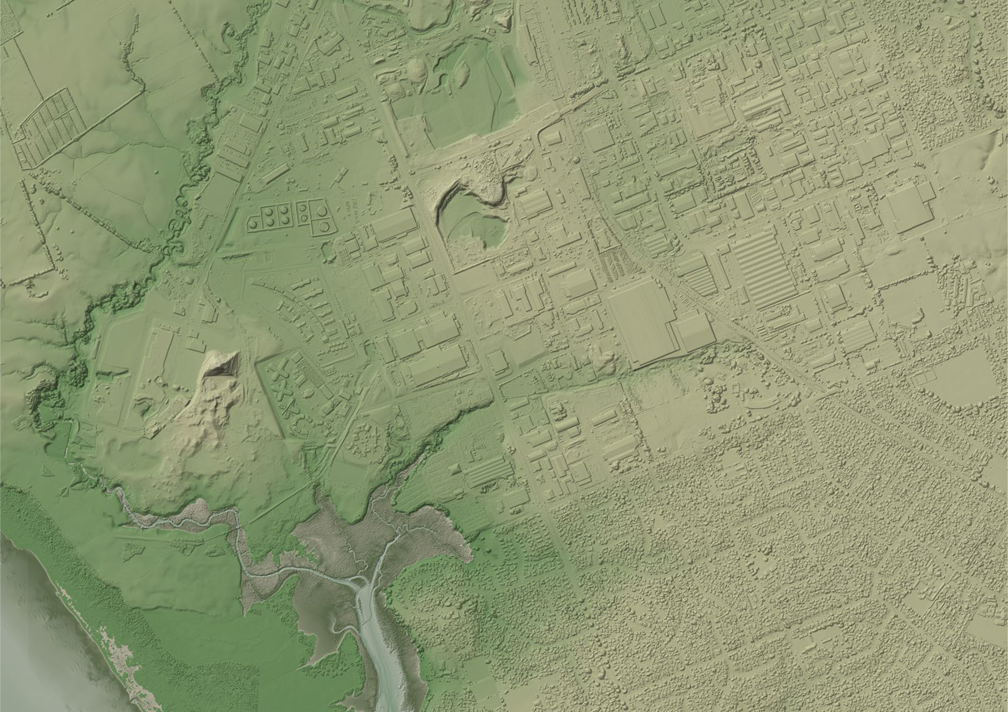
Finally, I needed an intertidal model. Since, there are a number of different intertidal zones represented around Auckland: estuaries, sandy beaches and rocky shores and I am using only one DEM, I needed to choose which intertidal zone to represent in the image. One colour gradient does not fit all. I had to make a choice. I decided to use the mud flats and estuaries as the primary intertidal model. The DEM included the channels in the mudflats and I really liked the shapes they made. They also covered wide areas and were a prominent feature. Img 2: Elevation model focusing on marshy tidal zones
With the intertidal model determined and the zones set, I developed the colour gradients.
| Elevation Value | Colour | Zone |
|---|---|---|
| -1.0 | Bathymetric | |
| -0.75 | Bathymetric | |
| 0.5 | Intertidal | |
| 1.0 | Intertidal | |
| 1.7 | Intertidal | |
| 1.8 | Terrestrial | |
| 25 | Terrestrial | |
| 100 | Terrestrial | |
| 500 | Terrestrial |
Note: The elevation values used do not necessarily correlate with the actual elevations where these zones transition. They are a best estimation based on samplings from aerial imagery.
Blending the Layers
For the final step, I blended the layers in QGIS. I needed the hillshades I developed from the DEM and DSM, plus the original DEM elevation. That’s it. Three layers for the whole thing. The DEM elevation carried all the colour work, the DSM hillshades gave the detail, and the DEM hillshade added some weight to the shaded areas. Here is the order and blending for the project in QGIS:
- DSM Hillshade: multiply, brightness 50%, black in hillshade set to #333333
- DEM Hillshade: multiply, brightness 50%
- DEM: contrast 10%
Overall, the base image proved to be a success and the script has been useful across a number of projects. The images have ended up in a good bit of internal and conference media and I have seen steady use for almost two years now. For me, the image is getting tired and I’d eventually love to redevelop the gradients; but, I am happy to have a chance to write about it and get some more external exposure. In the future, I am looking to develop this map a bit further and present it as a web map as well. Time will tell whether this happens or not. I think it would take a directive from an outside source.
I’d be keen to hear your comments below or get in touch if you are interested in learning more.
 Img 3: Promotional media
Note: All imagery was produced during my time at Land Information New Zealand. Imagery licensing can be found here:
“Source: Land Information New Zealand (LINZ) and licensed by LINZ for re-use under the Creative Commons Attribution 4.0 International licence.”