XYCarto

It is important to note something from the very beginning. The interpolated bathymetry developed in this project does not reflect the actual bathymetry of the Wellington Harbour. It is my best guess based on the tools I had and the data I worked with. Furthermore, this interpolation is NOT the official product of any institution. It is an interpolation created by me only for the purposes of visualization.

Part of the goal when visualizing the Wellington landscape was to incorporate a better idea about what may be happening below the surface of the harbor. Various bathymetric scans in the past have gathered much of the information and institutions like NIWA have done the work visualizing that data. As for myself, I did not have access to those bathymetries; however, I did have a sounding point data set to work with, so I set about interpolating those points.

The data set, in CSV format, was over a million points; too dense for a single interpolation. I worked out a basic plan for the interpolation based on splitting the points into a grid, interpolate the smaller bits, then reassemble the grid tiles into a uniform bathymetry.

Conversion from CSV to shp
Using the open option (-oo) switch, OGR will convert CSV to shp seamlessly

ogr2ogr -s_srs EPSG:4167 -t_srs EPSG:4167 -oo X_POSSIBLE_NAMES=$xname* -oo Y_POSSIBLE_NAMES=$yname*  -f "ESRI Shapefile" $outputshapepath/$basenme.shp $i

Gridding the Shapefile
With the shapefile in place, I next needed to break it into smaller pieces for interpolation. For now, I create the grid by hand in QGIS using the ‘Create Grid’ function. This is found under Vector>Reasearch Tools>Create Grid. Determining a grid size that works best for the interpolation is a bit of trial and error. You want the largest size your interpolation can manage without crashing. Using the grid tool from QGIS in very convenient, in that it creates an attribute table of the xmin, xmax, ymin, ymax corrodinates for each tile in the grid. These attributes become very helpful during the interpolation process.

Interpolating the Points
I switched things up in the interpolation methods this time and tried out SAGA GIS. I have been looking for a while now for a fast and efficient method of interpolation that I could easily build into a scripted process. SAGA seemed like a good tool for this. The only drawback, I had a very hard time finding examples online about how to use this tool. My work around to was to test the tool in QGIS first. I noticed when the command would run, QGIS saved the last command in a log file. I found that log, copied out the command line function, and began to build my SAGA command for my script from there.

Here is look at the command I used:

saga_cmd grid_spline "Multilevel B-Spline Interpolation" -TARGET_DEFINITION 0 -SHAPES "$inputpoints" -FIELD "depth" -METHOD 0 -EPSILON 0.0001 -TARGET_USER_XMIN $xmin -TARGET_USER_XMAX $xmax -TARGET_USER_YMIN $ymin -TARGET_USER_YMAX $ymax -TARGET_USER_SIZE $reso -TARGET_USER_FITS 0 -TARGET_OUT_GRID "$rasteroutput/sdat/spline_${i}"

I tested a number of methods and landed on ‘grid_spline’ as producing the best results for the project. It was useful because it did a smooth interpolation across the large ‘nodata’ spaces.

Once the initial interpolation was complete, I needed to convert the output to GeoTIFF since SAGA exports in an .sdat format. Easy enough since GDAL_TRANSLATE recognizes the .sdat format. I then did my standard prepping and formatting for visualization:

gdal_translate "$iupput_sdat/IDW_${i}.sdat" "$output_tif/IDW_${i}.tif"
gdaldem hillshade -multidirectional -compute_edges "$output_tif/IDW_${i}.tif" "$ouput_hs/IDW_${i}.tif"
gdaladdo -ro "$output_tif/IDW_${i}.tif" 2 4 8 16 32 64 128
gdaladdo -ro "$ouput_hs/IDW_${i}.tif"2 4 8 16 32 64 128

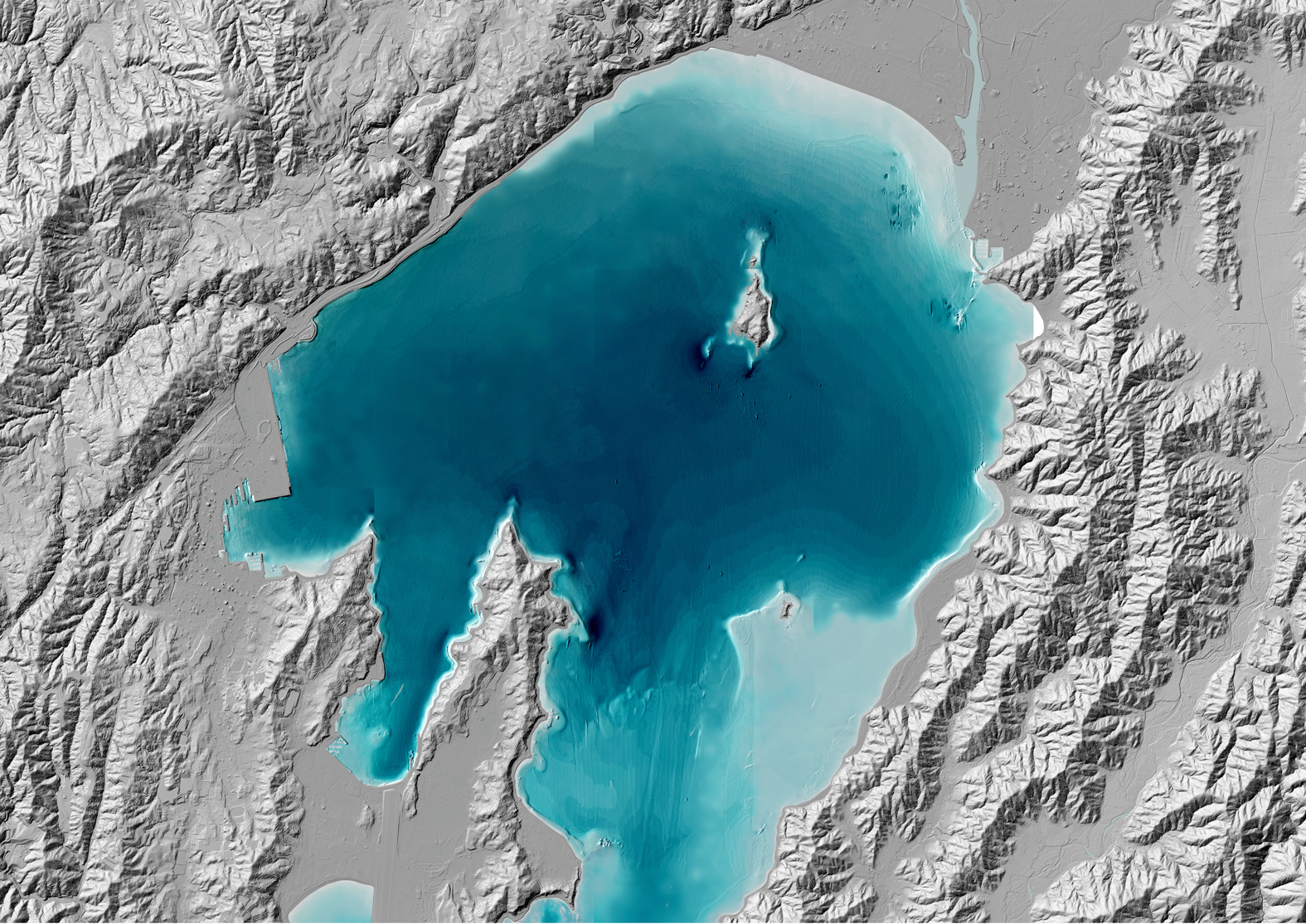
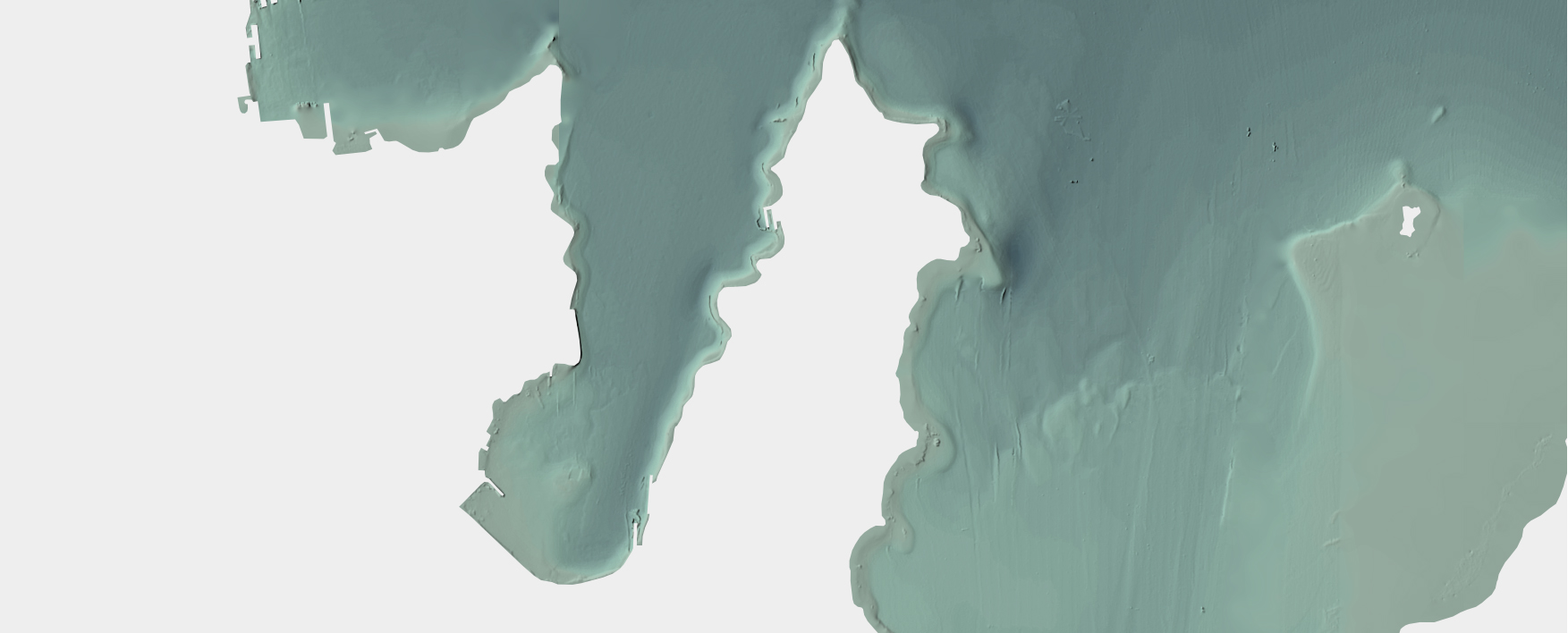
Here is look at the interpolated harbour bathymetry, hillshaded, with Wellington 1m DEM hillshade added over top

And here is a look at the same bathy hillshade with coloring

Visualizing the Bathymetry
The visualization is four steps:

Hillshade

Color

Aerial Imagery

Then merge the models together

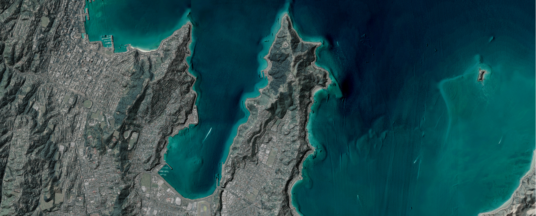
Easy as, eh? Let me know what you think!

Note: All imagery was produced during my time at Land Information New Zealand. Imagery licensing can be found here:
“Source: Land Information New Zealand (LINZ) and licensed by LINZ for re-use under the Creative Commons Attribution 4.0 International licence.”